Minimal working example
[1]:
import pandas as pd
import numpy as np

from mprod.dimensionality_reduction import TCAM
from mprod import table2tensor

import matplotlib.pyplot as plt
import seaborn as sns; sns.set_style('ticks')
%matplotlib inline
Load files
[2]:
file_path = "./data/Suez2018.txt"
data_raw = pd.read_csv(file_path, index_col=[0,1,2,3]
                       , dtype={'Participant':int,'Day':int})
meta_time = data_raw.index.to_frame().reset_index(drop = True)
meta = meta_time.drop(['Day','Phase'], axis=1).drop_duplicates()

display(data_raw.head())
display(meta_time.head())
display(meta.head())
| s__Vagococcus_lutrae | s__Asaccharobacter_celatus | s__Megasphaera_elsdenii | s__Leuconostoc_carnosum | s__Streptococcus_agalactiae | s__Tyzzerella_nexilis | s__Akkermansia_muciniphila | s__Alistipes_timonensis | s__Peptostreptococcus_anaerobius | s__Streptococcus_anginosus_group | ... | s__Clostridium_celatum | s__Fusobacterium_periodonticum | s__Acidaminococcus_intestini | s__Streptococcus_sobrinus | s__Anaerostipes_caccae | s__Enterococcus_faecium | s__Eubacterium_sp_CAG_180 | s__Veillonella_dispar | s__Actinomyces_sp_S6_Spd3 | s__Firmicutes_bacterium_CAG_238 | ||||
|---|---|---|---|---|---|---|---|---|---|---|---|---|---|---|---|---|---|---|---|---|---|---|---|---|
| Participant | Phase | Group | Day | |||||||||||||||||||||
| 602 | BAS | FMT | 3 | 9.999999e-07 | 0.000051 | 0.018276 | 9.999999e-07 | 9.999999e-07 | 9.999999e-07 | 0.000198 | 9.999999e-07 | 9.999999e-07 | 9.999999e-07 | ... | 9.999999e-07 | 9.999999e-07 | 2.247164e-04 | 9.999999e-07 | 9.999999e-07 | 9.999999e-07 | 0.005217 | 9.999999e-07 | 9.999999e-07 | 5.632903e-05 |
| 6 | 9.999999e-07 | 0.000263 | 0.017956 | 9.999999e-07 | 9.999999e-07 | 9.999999e-07 | 0.000175 | 9.999999e-07 | 9.999999e-07 | 9.999999e-07 | ... | 9.586594e-05 | 9.999999e-07 | 3.205194e-04 | 9.999999e-07 | 9.999999e-07 | 9.999999e-07 | 0.005515 | 9.999999e-07 | 9.999999e-07 | 9.263375e-05 | |||
| ABX | FMT | 10 | 1.000001e-06 | 0.000001 | 0.000001 | 1.000001e-06 | 1.000001e-06 | 1.000001e-06 | 0.000001 | 1.000001e-06 | 1.000001e-06 | 2.271773e-03 | ... | 1.000001e-06 | 1.000001e-06 | 1.000001e-06 | 1.000001e-06 | 1.000001e-06 | 1.000001e-06 | 0.000001 | 1.000001e-06 | 1.000001e-06 | 1.000001e-06 | |
| 13 | 1.000000e-06 | 0.000012 | 0.000270 | 1.000000e-06 | 1.000000e-06 | 1.000000e-06 | 0.000209 | 1.000000e-06 | 1.000000e-06 | 1.298585e-03 | ... | 1.000000e-06 | 1.000000e-06 | 1.000000e-06 | 1.000000e-06 | 1.000000e-06 | 5.046216e-04 | 0.001349 | 1.000000e-06 | 1.000000e-06 | 1.000000e-06 | |||
| INT | FMT | 17 | 9.999999e-07 | 0.000027 | 0.000628 | 9.999999e-07 | 9.999999e-07 | 9.999999e-07 | 0.000486 | 9.999999e-07 | 9.999999e-07 | 9.999999e-07 | ... | 9.999999e-07 | 9.999999e-07 | 9.999999e-07 | 9.999999e-07 | 9.999999e-07 | 1.176117e-03 | 0.003147 | 9.999999e-07 | 9.999999e-07 | 9.999999e-07 |
5 rows × 482 columns
| Participant | Phase | Group | Day | |
|---|---|---|---|---|
| 0 | 602 | BAS | FMT | 3 |
| 1 | 602 | BAS | FMT | 6 |
| 2 | 602 | ABX | FMT | 10 |
| 3 | 602 | ABX | FMT | 13 |
| 4 | 602 | INT | FMT | 17 |
| Participant | Group | |
|---|---|---|
| 0 | 602 | FMT |
| 9 | 603 | FMT |
| 18 | 604 | FMT |
| 27 | 605 | FMT |
| 36 | 606 | FMT |
Data normalization and mode-mapping
[3]:
data_normalized = data_raw.groupby(level = 'Participant' )\
                    .apply(lambda x:np.log2(x/x.query("Phase == 'BAS'").mean()))
data_normalized = data_normalized.reset_index(level=['Phase','Group']
                                              , drop = True)
display(data_normalized.head())
| s__Vagococcus_lutrae | s__Asaccharobacter_celatus | s__Megasphaera_elsdenii | s__Leuconostoc_carnosum | s__Streptococcus_agalactiae | s__Tyzzerella_nexilis | s__Akkermansia_muciniphila | s__Alistipes_timonensis | s__Peptostreptococcus_anaerobius | s__Streptococcus_anginosus_group | ... | s__Clostridium_celatum | s__Fusobacterium_periodonticum | s__Acidaminococcus_intestini | s__Streptococcus_sobrinus | s__Anaerostipes_caccae | s__Enterococcus_faecium | s__Eubacterium_sp_CAG_180 | s__Veillonella_dispar | s__Actinomyces_sp_S6_Spd3 | s__Firmicutes_bacterium_CAG_238 | ||
|---|---|---|---|---|---|---|---|---|---|---|---|---|---|---|---|---|---|---|---|---|---|---|
| Participant | Day | |||||||||||||||||||||
| 602 | 3 | -8.872499e-09 | -1.623746 | 0.012707 | -8.872499e-09 | -8.872499e-09 | -8.872499e-09 | 0.086871 | -8.872499e-09 | -8.872499e-09 | -8.872499e-09 | ... | -5.597918 | -8.872499e-09 | -0.278775 | -8.872499e-09 | -8.872499e-09 | -8.872499e-09 | -0.040705 | -8.872499e-09 | -8.872499e-09 | -0.403001 |
| 6 | 8.872499e-09 | 0.744599 | -0.012820 | 8.872499e-09 | 8.872499e-09 | 8.872499e-09 | -0.092439 | 8.872499e-09 | 8.872499e-09 | 8.872499e-09 | ... | 0.985029 | 8.872499e-09 | 0.233532 | 8.872499e-09 | 8.872499e-09 | 8.872499e-09 | 0.039588 | 8.872499e-09 | 8.872499e-09 | 0.314658 | |
| 10 | 1.337567e-06 | -7.295634 | -14.144966 | 1.337567e-06 | 1.337567e-06 | 1.337567e-06 | -7.542312 | 1.337567e-06 | 1.337567e-06 | 1.114960e+01 | ... | -5.597916 | 1.337567e-06 | -8.090735 | 1.337567e-06 | 1.337567e-06 | 1.337567e-06 | -12.389628 | 1.337567e-06 | 1.337567e-06 | -6.218807 | |
| 13 | 7.558580e-07 | -3.707767 | -6.069695 | 7.558580e-07 | 7.558580e-07 | 7.558580e-07 | 0.164989 | 7.558580e-07 | 7.558580e-07 | 1.034272e+01 | ... | -5.597917 | 7.558580e-07 | -8.090736 | 7.558580e-07 | 7.558580e-07 | 8.979058e+00 | -1.991681 | 7.558580e-07 | 7.558580e-07 | -6.218808 | |
| 17 | -1.975416e-08 | -2.555618 | -4.850362 | -1.975416e-08 | -1.975416e-08 | -1.975416e-08 | 1.383432 | -1.975416e-08 | -1.975416e-08 | -1.975416e-08 | ... | -5.597918 | -1.975416e-08 | -8.090737 | -1.975416e-08 | -1.975416e-08 | 1.019982e+01 | -0.769899 | -1.975416e-08 | -1.975416e-08 | -6.218808 |
5 rows × 482 columns
[4]:
tensor_data, mode1_map, mode3_map = table2tensor(data_normalized)
mode1_reverse_map = {val:k for k,val in mode1_map.items()}

display(tensor_data.shape)
print(mode1_map)
print(mode1_reverse_map)
(17, 482, 9)
{602: 0, 603: 1, 604: 2, 605: 3, 606: 4, 701: 5, 702: 6, 703: 7, 704: 8, 707: 9, 708: 10, 801: 11, 802: 12, 803: 13, 804: 14, 806: 15, 807: 16}
{0: 602, 1: 603, 2: 604, 3: 605, 4: 606, 5: 701, 6: 702, 7: 703, 8: 704, 9: 707, 10: 708, 11: 801, 12: 802, 13: 803, 14: 804, 15: 806, 16: 807}
Transform
The TCAM transformation is done by calling .fit and .transform methods of a TCAM object.
The TCAM class implements scikit-learn’s transformer-mixin methods, so its API is rather similar to sklearn’s PCA.
[5]:
tcam = TCAM(n_components=1.) # will produce all components
transformed_data = tcam.fit_transform(tensor_data)
rounded_expvar = np.round(100*tcam.explained_variance_ratio_,2) # store explained variance ratios
# cast the results data into a pandas dataframe, using the first mode identifiers (subjects)
# as indices (row names)
df_tca = pd.DataFrame(transformed_data).rename(index = mode1_reverse_map)
df_tca.columns = [f'F{i}:{val}%' for i,val in enumerate(rounded_expvar, start = 1)]
# append metadata to the factors dataframe
df_plot = meta.merge(df_tca, left_on = 'Participant', right_index=True)
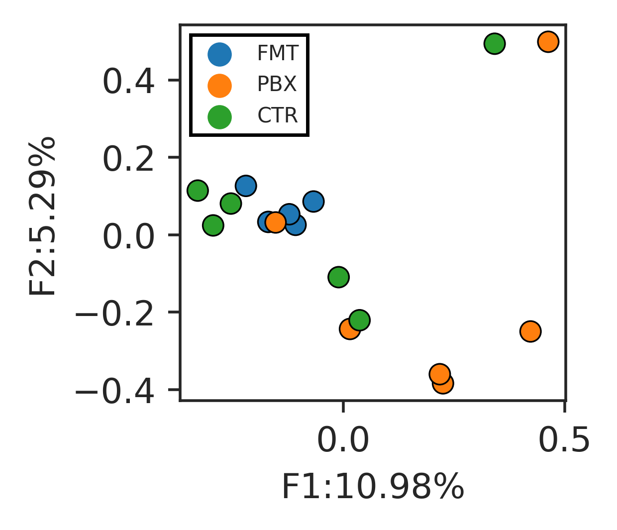
f1, f2 = df_tca.columns[:2].tolist() # get the column names for the first 2 factors
fig, ax = plt.subplots(figsize = [2,2], dpi = 500)
sns.scatterplot(data = df_plot, x = f1, y = f2 , hue='Group', ax = ax, edgecolor = 'k')
ax.legend(fontsize = 6, fancybox = False, framealpha = 1, edgecolor = 'k' )
plt.show()
[ ]: