Supervised learning¶

Supervised ML is the task of learning a function that maps an input to an output based on example input-output pairs. Formally, we are given with a set \(\mathcal{D}\) consists of (data,labels) pairs:

\[\mathcal{D} = \{ (x_i , y_i) \}_{i=1}^{m}\]

where \(x_i \in \mathcal{X}\) are the datapoints and \(y_i \in \mathcal{Y}\) are the labels. For simplicity, we assume here that the “labels space” \(\mathcal{Y}\) is a finite set \(y_i\) that are discrete, univariate variables, i.e., classification settings.

The goal in supervised learning is to fit a function \(f : \mathcal{X} \to \mathcal{Y}\) such that \(f(x_i) =y_i\) for all \(i=1,\dots,m\) . Traditionaly, the data points \(x_i\) are elements of some vector space, meaning that, each point can be expressed using a \(p\)-tuple (vector) of numbers

\[x_i = (x_{i1}, x_{i2}, \dots, x_{ip})\]

hence we have \(f : \mathbb{R}^p \to \mathcal{Y}\). However, when working with multi-way data, and time-series data in particular, the situation is different.

The case of matrix valued inputs¶

To adhere with the empirical results and demonstrations shown in 1, we restrict the discussion to the case where data points are gathered across multiple timepoints. That is, each sample \(x_i\) is in fact, an \(n\) by \(p\) matrix, where each of the \(p\) columns represents a feature and the rows correspond to different timepoints in which the samples were gathered.

The matrix input setting is not uncommon, for example, consider the task of gray-scale image classification, where each image is a set of \(n \times p\) pixels and each pixel holds a value from 0 to 1 determining its brightness. In the case of longitudinal sampling data, we can think of the rows of each sample \(x_i\) as discrete samples of a “curve” in a \(p\) dimensional space. In formal words, let \(\gamma_i : \mathbb{R} \to \mathbb{R}^p\) a smooth function, and \(\{t_j\}_{j=1}^n \subset \mathbb{R}\) be a set of timepoints, such that \(\gamma_i (t_j) \in \mathbb{R}^p\) is the \(j^{th}\) row of the matrix \(x_i\) .

An illustration of the \(p\) dimensional curve \(\gamma_i\) (here \(p=3\)), were the blue line is the curve itself, points illustrate discrete sampling process, each point correspond to a timepoint \(t_j\) for \(j=1,\dots ,n\).¶

In our context, we are given with collection of such labeled curves, all of which are sampled in corresponding timepoints, and our goal is to fit a function that takes a sampled curve \(x =[\gamma (t_1), \gamma (t_2) , \dots , \gamma (t_n)]\) and outputs the label associated with the curve.

Illustration of the supervised curve classification task, curves are colored according to their class label.¶

ML workflows¶

The function \(f: \mathbb{R}^{n \times p} \to \mathcal{Y}\) usually consists of a composition of “simpler” functions

\[f(x) = f_1 \circ f_2 \circ ... \circ f_d (x)\]

i.e., a pipeline of functions, where each function \(f_j\) “captures” a certain property of the data that is key for making an accurate prediction, and such that the mapping \(f_j\) is vector valued, starting some \(j \leq d\) . Meaning that \(f_k (x) \in \mathbb{R}^{\ell_k}\) for all \(k\geq j\) . Examples for common functions of use in supevised ML are

In neural networks, \(f_j\) are of the form \(f_j (x) = \alpha_j ({\bf W}_j x + b_j)\) where
- \({\bf W}_j\) is a matrix representing a \(\mathbb{R}^{j_1} \to \mathbb{R}^{j_2}\) linear mapping
- \(b_j \in \mathbb{R}^{j_2}\) is a bias term
- \(\alpha_j\) is a non-linear activation function such as, \(\tanh, \operatorname{SoftMax} , \operatorname{sigmoid}\) etc…
Normalization steps, such as standard-scaling
Dimensionality reduction steps, like PCA, CCA, UMAM, etc…

An essential requirement we impose on the functions \(f_j\) is that after the training process is done, and the parameters are learned, each \(f_j\) must be applicable to samples outside of the training set \(\mathcal{D}\) .

Example

✔ Consider PCA as a dimensionality reduction step, then \(f_j (x) = x {\bf W}_j\) where entries of the matrix \({\bf W}_j\) are determined by the dataset \({\bf X} = [x_1 ; x_2 ; \dots ; x_m]\). Given a new data point \(\bar{x}\), the application of \(f_j\) to \(\bar{x}\) is done by simple matrix multiplication. n

✘ Alternatively, consider the mapping \(f_j\) obtained by fitting a PCoA (or multidimensional scaling) with respect to some dissimilarity funtion. Then the mapping \(f_j\) is relevant only to the samples that are in the training dataset. Applying it as a transformation to samples outside \(\mathcal{D}\) is not straight forward.

In our terminology, functions that are easily applied to data outside of the training dataset are called out-of-sample extendable.

TCAM as dimensionality reduction step¶

The TCAM is a \(\mathbb{R}^{n \times p} \to \mathbb{R}^q\) mapping that is

✔ Variance maximizing (*)
✔ Distortion minimizing (*)
✔ Out-of-sample extendable

It makes perfect sense to use it as a dimensionality reduction step within ML workflows.

(*) within the set of pseudo- \(\star_{\bf M}\) orthogonal mappings of rank \(q\) 1

Concrete example¶

We will now construct a concrete example for the incorporation of TCAM in supervised ML workflow for curve classification, using real world microbiome data.

Dataset¶

The data in the following example was obtained from a study by Schirmer et al. 2 . In this study, the authors charactarized the gut microbiome throughout a disease course for 405 pediatric, new-onset, treatment-naive ulcerative colitis (UC) patients.

Patients were monitored for 1 year upon treatment initiation, and microbial taxonomic composition was analyzed from fecal samples using 16S rRNA gene amplicon sequencing. Fecal samples were collected at baseline (week 0, prior to treatment) and 3 follow-up time points (4, 12, and 52 weeks after treatment initiation). At the end of the year, patients were assigned with “label” according their disease state, that is either “Flare” or “Remission”.

Formally:

Inputs: \(\mathcal{X} \subset \mathbb{R}^{n \times p}\) where \(n\) are the four time points, and \(p\) are the number of features obtained by 16S metagenomics sequencing.
Labels: \(\mathcal{Y} = \{ \operatorname{Flare}, \operatorname{Remission} \}\)

We read the data from our git repository as follows

[1]:

import pandas as pd
import numpy as np

data_raw = pd.read_csv("https://raw.githubusercontent.com/UriaMorP/"
                       "tcam_analysis_notebooks/main/Schirmer2018/Schirmer2018.tsv"
                       , index_col=[0,1], sep="\t"
                       , dtype={'Week':int})


labels = pd.read_csv("https://raw.githubusercontent.com/UriaMorP/"
                   "tcam_analysis_notebooks/main/Schirmer2018/metadata_Schirmer2018.tsv"
                   , index_col=[0], sep="\t").loc[data_raw.index.get_level_values(0), 'Remission'].rename('label')
labels = 1 * (labels == "Remission") # Binarize the labels
labels = labels.reset_index().copy()


print("Data")
display(data_raw.head(12))
print("Labels")
display(labels.head(4))

Data

		k__Bacteria-p__Firmicutes-c__Clostridia-o__Clostridiales-f__Ruminococcaceae-g__Oscillospira-s__-OTU_310886	k__Bacteria-p__Firmicutes-c__Clostridia-o__Clostridiales-f__Peptostreptococcaceae-g__-s__-OTU_531374	k__Bacteria-p__Firmicutes-c__Clostridia-o__Clostridiales-f__-g__-s__-OTU_366584	k__Bacteria-p__Proteobacteria-c__Betaproteobacteria-o__Burkholderiales-f__Alcaligenaceae-g__Sutterella-s__-OTU_173726	k__Bacteria-p__Firmicutes-c__Clostridia-o__Clostridiales-f__Ruminococcaceae-g__-s__-OTU_366794	k__Bacteria-p__Firmicutes-c__Clostridia-o__Clostridiales-f__Lachnospiraceae-g__-s__-OTU_975306	k__Bacteria-p__Bacteroidetes-c__Bacteroidia-o__Bacteroidales-f__Porphyromonadaceae-g__Parabacteroides-s__distasonis-OTU_585914	k__Bacteria-p__Firmicutes-c__Clostridia-o__Clostridiales-f__-g__-s__-OTU_352304	k__Bacteria-p__Firmicutes-c__Clostridia-o__Clostridiales-f__Lachnospiraceae-g__Blautia-s__-OTU_193061	k__Bacteria-p__Bacteroidetes-c__Bacteroidia-o__Bacteroidales-f__Prevotellaceae-g__Prevotella-s__-OTU_4302472	...	k__Bacteria-p__Firmicutes-c__Clostridia-o__Clostridiales-f__Lachnospiraceae-g__Roseburia-s__-OTU_313593	k__Bacteria-p__Synergistetes-c__Synergistia-o__Synergistales-f__-g__-s__-OTU_505549	k__Bacteria-p__Actinobacteria-c__Coriobacteriia-o__Coriobacteriales-f__Coriobacteriaceae-g__-s__-OTU_4403259	k__Bacteria-p__Firmicutes-c__Clostridia-o__Clostridiales-f__Lachnospiraceae-g__Epulopiscium-s__-OTU_4371562	k__Bacteria-p__Bacteroidetes-c__Bacteroidia-o__Bacteroidales-f__S24.7-g__-s__-OTU_1115121	k__Bacteria-p__Firmicutes-c__Clostridia-o__Clostridiales-f__Ruminococcaceae-g__-s__-OTU_300870	k__Bacteria-p__Bacteroidetes-c__Bacteroidia-o__Bacteroidales-f__Porphyromonadaceae-g__Parabacteroides-s__distasonis-OTU_186233	k__Bacteria-p__Firmicutes-c__Clostridia-o__Clostridiales-f__Lachnospiraceae-g__.Ruminococcus-.s__-OTU_300877	k__Bacteria-p__Firmicutes-c__Clostridia-o__Clostridiales-f__.Tissierellaceae-.g__-s__-OTU_869796	k__Bacteria-p__Firmicutes-c__Clostridia-o__Clostridiales-f__Ruminococcaceae-g__Ruminococcus-s__-OTU_196061
SubjectID	Week
P_10343	0	0.000000	0.000000	0.000000	0.0	0.0	0.000869	0.022900	0.000033	0.000000	0.0	...	0.000000	0.000000	0.0	0.0	0.000000	0.0	0.0	0.000000	0.0	0.0
	4	0.000183	0.000000	0.008966	0.0	0.0	0.020421	0.000000	0.000823	0.000000	0.0	...	0.000073	0.000000	0.0	0.0	0.000000	0.0	0.0	0.000000	0.0	0.0
	12	0.000000	0.000000	0.000000	0.0	0.0	0.006230	0.000049	0.000997	0.000000	0.0	...	0.000049	0.000000	0.0	0.0	0.000000	0.0	0.0	0.000000	0.0	0.0
	52	0.000000	0.000097	0.000000	0.0	0.0	0.002211	0.000000	0.000291	0.000000	0.0	...	0.000000	0.000000	0.0	0.0	0.000000	0.0	0.0	0.000048	0.0	0.0
P_10897	0	0.000423	0.000000	0.000059	0.0	0.0	0.077260	0.000863	0.017448	0.000051	0.0	...	0.000008	0.000000	0.0	0.0	0.000000	0.0	0.0	0.000000	0.0	0.0
	4	0.000023	0.000000	0.000000	0.0	0.0	0.006095	0.000411	0.000000	0.000000	0.0	...	0.000000	0.000000	0.0	0.0	0.000000	0.0	0.0	0.000000	0.0	0.0
	12	0.000080	0.000013	0.010809	0.0	0.0	0.005411	0.000372	0.000359	0.000027	0.0	...	0.000027	0.000000	0.0	0.0	0.000000	0.0	0.0	0.000000	0.0	0.0
	52	0.000000	0.000080	0.000664	0.0	0.0	0.013934	0.000261	0.000905	0.000000	0.0	...	0.000040	0.000000	0.0	0.0	0.000000	0.0	0.0	0.000000	0.0	0.0
P_1108	0	0.000000	0.000000	0.000000	0.0	0.0	0.002086	0.000000	0.000066	0.000016	0.0	...	0.000049	0.000000	0.0	0.0	0.000049	0.0	0.0	0.000000	0.0	0.0
	4	0.000000	0.000211	0.000000	0.0	0.0	0.011007	0.000000	0.000409	0.000000	0.0	...	0.000384	0.000025	0.0	0.0	0.000000	0.0	0.0	0.000000	0.0	0.0
	12	0.000007	0.000000	0.000028	0.0	0.0	0.038760	0.000528	0.003105	0.000000	0.0	...	0.000428	0.000000	0.0	0.0	0.000000	0.0	0.0	0.000000	0.0	0.0
	52	0.000000	0.000000	0.000000	0.0	0.0	0.115325	0.002798	0.018651	0.000000	0.0	...	0.000311	0.000000	0.0	0.0	0.000000	0.0	0.0	0.000000	0.0	0.0

12 rows × 1015 columns

Labels

	SubjectID	label
0	P_10343	0
1	P_10343	0
2	P_10343	0
3	P_10343	0

Making the ML workflow¶

We rely on sklearn’s Pipeline interface in order to implement the composition of functions, previously formulated as \(f = f_1 \circ f_2 \circ ... \circ f_d\) making the classification model.

A python code realization of the above mathematical formulation would be as follows:

from sklearn.pipeline import Pipeline

pipe = Pipeline([
    ('f_1', Transformer1())
    ,('f_2', Transformer2())
    # ...
    ,('f_d', Estimator())
])

where Transformers are classes implementing sklearn.base.TransformerMixin and Estimator implements sklearn.base.BaseEstimator .

In this example, we use the following steps

Filtration of low-abundant features
Curvewise standardization
TCAM truncation
MinMax scaling
GradientBoostClassifier

For steps 1.-3. it is most convenient to work with pandas.DataFrames as inputs.

[2]:

from sklearn.base import BaseEstimator, TransformerMixin

# step 1: Filtration of low-abundant features
class RAFilter(BaseEstimator, TransformerMixin):
    def __init__(self, capval = 5e-2):
        self._f_list = []
        self.capval = capval
        pass

    def fit(self, X,y=None, modemap = []):
        X_t = X.copy()
        X_t = 100 * (X_t / X_t.values.sum(axis=1,keepdims = True))
        self._f_list = [i for i in range(X_t.shape[1]) if (X_t.iloc[:,i] > self.capval).sum() > X_t.shape[0]*0.1 ]
        return self

    def transform(self, X, y = None):
        X_t = 100 * (X / X.values.sum(axis=1,keepdims = True)).copy()
        X_t = X_t.iloc[:,self._f_list]
        X_t[X_t < self.capval] = self.capval
        X_t = 100 * X_t / X_t.values.sum(axis=1,keepdims = True)
        return X_t

    def fit_transform(self, X, y = None, modemap = []):
        self = self.fit(X, y)
        Xt = self.transform(X, y)
        return Xt

Since microbiome data tends to cluster by participant, meaning that variation coming from interindividual differences tend overshadow any other source of variation, including temporal trends, the task of identifying mutual temporal trajectories in microbiome composition is very challenging. Keeping in mind that we are only concerned with the direction of temporal variation trends (rather than the concrete baseline), one simple way of tackling this challenge would be to look at deviations from the baseline period. That is, instead of looking at raw values \(x_{ij}\) (the \(j^{th}\) time point of subject \(i\)), we consider tthe followoing:

\[z_{ij} = \log_{2}(x_{ij} / \mu(x_{i0}) )\]

where \(\mu ( x_{i0} )\) denotes the baseline sample of subject \(i\) . Using pandas, this transfromation looks like:

[3]:

from sklearn.preprocessing import FunctionTransformer

# step 2: Curvewise standardization
def standardize_curve_df(X, y = None, cap = 5e-3):
    blmean = (X + cap).groupby(level=['SubjectID']).apply(lambda x:x / x.loc[x.index.get_level_values('Week') == 0].iloc[0] )
    blmean = np.log2(blmean)
    return blmean

# Wrap the function with Transformer
StandardCurve = FunctionTransformer(standardize_curve_df)

Step 3. is the last step applied to a dataframe. In this step, we cast the dataframe into a tensor, then a TCAM is applied, followed by truncation (dimensionality reduction step) and a numpy.array is returned.

Gotcha

Suppose that the size of the training dataset is \(4m\) in its tabular form, the number of rows in the output of TCAMWrapper.transform is \(m\)

For many good reasons, this reduction in number of samples , is not allowed by the Pipeline (it throws a ValueError: Found input variables with inconsistent numbers of samples: [m, 4m] )

In our case, this decrease is intentional, and we hack our way around sklearn’s safeguards

To overcome this inconsistency, we divide the workflow into two pipelines each of which maintains consistent number of rows, and the TCAM transformation is patched between the two pipelines.

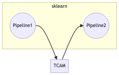
The pipeline patching process, the inputs and outputs of Pipeline1 all have \(4m\) rows, while those of Pipeline1 have \(m\) rows. The TCAM transformation (of matrix to tensors) takes inputs with \(4m\) rows and outputs tables of \(m\) rows.¶

[4]:

from sklearn.pipeline import Pipeline
from sklearn.preprocessing import MinMaxScaler
from sklearn.neural_network import MLPClassifier
from sklearn.ensemble  import RandomForestClassifier, GradientBoostingClassifier
from mprod.dimensionality_reduction import TCAM
from mprod import table2tensor

class Patch(BaseEstimator, TransformerMixin):
    def __init__(self,pipeline1, tcam_obj):
        self.pipeline1 = pipeline1
        self.tcam_obj = tcam_obj

    def _transform_y(self, y, map1):
        yt = pd.Series(map1).rename('row').to_frame()
        yt = yt.merge(y.reset_index(), left_index = True, right_on = "SubjectID").drop_duplicates()
        yt.index = yt['row']
        yt = yt['label'].sort_index()
        return yt


    def fit(self, X, y = None):
        self.pipeline1 = self.pipeline1.fit(X,y=y)
        tensor, map1, map3 = table2tensor(self.pipeline1.transform(X))

        if y is not None:
            yt = self._transform_y(y,map1)
        else:
            yt = None

        self.tcam_obj = self.tcam_obj.fit(tensor,y=yt)
        return self

    def transform(self, X):
        Xt1 = self.pipeline1.transform(X)
        tensor, map1, map3 = table2tensor(Xt1)
        Xt2 = self.tcam_obj.transform(tensor)
        return Xt2

Instantiation on this workflow is done as follows:

[5]:

rs = 0      # To make sure executions are consistant
pipeline1 = Pipeline([
    ("raf", RAFilter(capval = 5e-3)),
    ("st_curve", StandardCurve)
])

pipeline2 = Pipeline([
    ('mmt',MinMaxScaler(clip = True)),
    ('clf', GradientBoostingClassifier(learning_rate=.2,random_state=rs))
])

patch = Pipeline([
    ('pipeline1',Patch(pipeline1, TCAM(n_components=.8)))
    , ('pipeline2', pipeline2)])

Fron here and on, the patch object is just like any other classification model, and can be evaluated as such

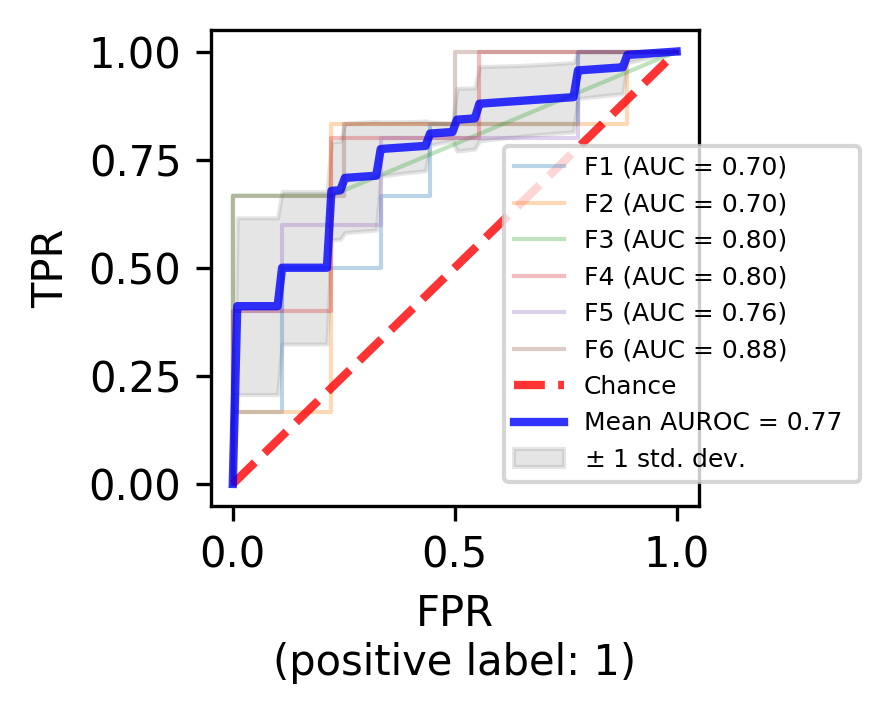
Model evaluation¶

[6]:

from sklearn.model_selection import StratifiedKFold
from sklearn.metrics import auc
from sklearn.metrics import plot_roc_curve, roc_curve
import matplotlib.pyplot as plt
%matplotlib inline

cv = StratifiedKFold(n_splits=6, shuffle=True, random_state=rs)

# indices for CV iterations
sid_ser = labels.copy().drop_duplicates()
sid_ser.index = sid_ser['SubjectID']
sid_ser = sid_ser['label']
dummy_size = np.arange(sid_ser.values.size)

# storing the model's scores
tprs = []
aucs = []
mean_fpr = np.linspace(0, 1, 100)

# CV loop
fig, ax = plt.subplots()
for i, (train_iloc, test_iloc) in enumerate(cv.split(dummy_size,sid_ser.values, sid_ser.values)):

    train_id = sid_ser.index[train_iloc].copy().sort_values()
    test_id = sid_ser.index[test_iloc].copy().sort_values()

    y_train = sid_ser[train_id].copy()
    X_train = data_raw.loc[data_raw.index.get_level_values("SubjectID").isin(y_train.index)].copy().sort_index(0)

    y_test = sid_ser[test_id].copy()
    X_test = data_raw.loc[data_raw.index.get_level_values("SubjectID").isin(y_test.index)].copy().sort_index(0)

    trained_model = patch.fit(X_train, y_train.copy())
    viz = plot_roc_curve(trained_model, X_test, y_test.copy(),
                     name='F{}'.format(i+1),
                     alpha=0.3, lw=1, ax=ax)

    interp_tpr = np.interp(mean_fpr, viz.fpr, viz.tpr)
    interp_tpr[0] = 0.0

    tprs.append(interp_tpr)
    aucs.append(viz.roc_auc)

ax.plot([0, 1], [0, 1], linestyle="--", lw=2, color="r", label="Chance", alpha=0.8)

mean_tpr = np.mean(tprs, axis=0)
mean_tpr[-1] = 1.0
mean_auc = auc(mean_fpr, mean_tpr)
std_auc = np.std(aucs)
ax.plot(
    mean_fpr,
    mean_tpr,
    color="b",
    label=r"Mean AUROC = %0.2f " % (mean_auc),
    lw=2,
    alpha=0.8,
)

std_tpr = np.std(tprs, axis=0)
tprs_upper = np.minimum(mean_tpr + std_tpr, 1)
tprs_lower = np.maximum(mean_tpr - std_tpr, 0)
ax.fill_between(
    mean_fpr,
    tprs_lower,
    tprs_upper,
    color="grey",
    alpha=0.2,
    label=r"$\pm$ 1 std. dev.",
)

ax.set(
    xlim=[-0.05, 1.05],
    ylim=[-0.05, 1.05],
)
ax.legend(loc=[.6, 0.05], fontsize = 6 )
ax.set_ylabel("TPR")
ax.set_xlabel("FPR\n(positive label: 1)")
fig.set_size_inches([2.1,2.1])
fig.set_dpi(300)
plt.show()

../_images/examples_supervised_learning_22_0.png

1(1,2): Uria Mor, Yotam Cohen, Rafael Valdes-Mas, Denise Kviatcovsky, Eran Elinav, and Haim Avron. Dimensionality reduction of longitudinal ‘omics data using modern tensor factorization. 2021. arXiv:2111.14159.
2: Melanie Schirmer, Lee Denson, Hera Vlamakis, Eric A. Franzosa, Sonia Thomas, Nathan M. Gotman, Paul Rufo, Susan S. Baker, Cary Sauer, James Markowitz, Marian Pfefferkorn, Maria Oliva-Hemker, Joel Rosh, Anthony Otley, Brendan Boyle, David Mack, Robert Baldassano, David Keljo, Neal LeLeiko, Melvin Heyman, Anne Griffiths, Ashish S. Patel, Joshua Noe, Subra Kugathasan, Thomas Walters, Curtis Huttenhower, Jeffrey Hyams, and Ramnik J. Xavier. Compositional and Temporal Changes in the Gut Microbiome of Pediatric Ulcerative Colitis Patients Are Linked to Disease Course. Cell Host & Microbe, 24(4):600–610.e4, oct 2018. URL: https://linkinghub.elsevier.com/retrieve/pii/S1931312818304931, doi:10.1016/j.chom.2018.09.009.